Interpretation of Connectivity Patterns
The results of this study confirm the hypothesis that the Canton of Schaffhausen functions as a highly fragmented landscape for large mammals. The resistance surface and subsequent LCP analysis highlight that ecological connectivity for Roe Deer is not limited by physical distance, but by the permeability of the anthropogenic matrix.
Network Topology and Funneling Effects
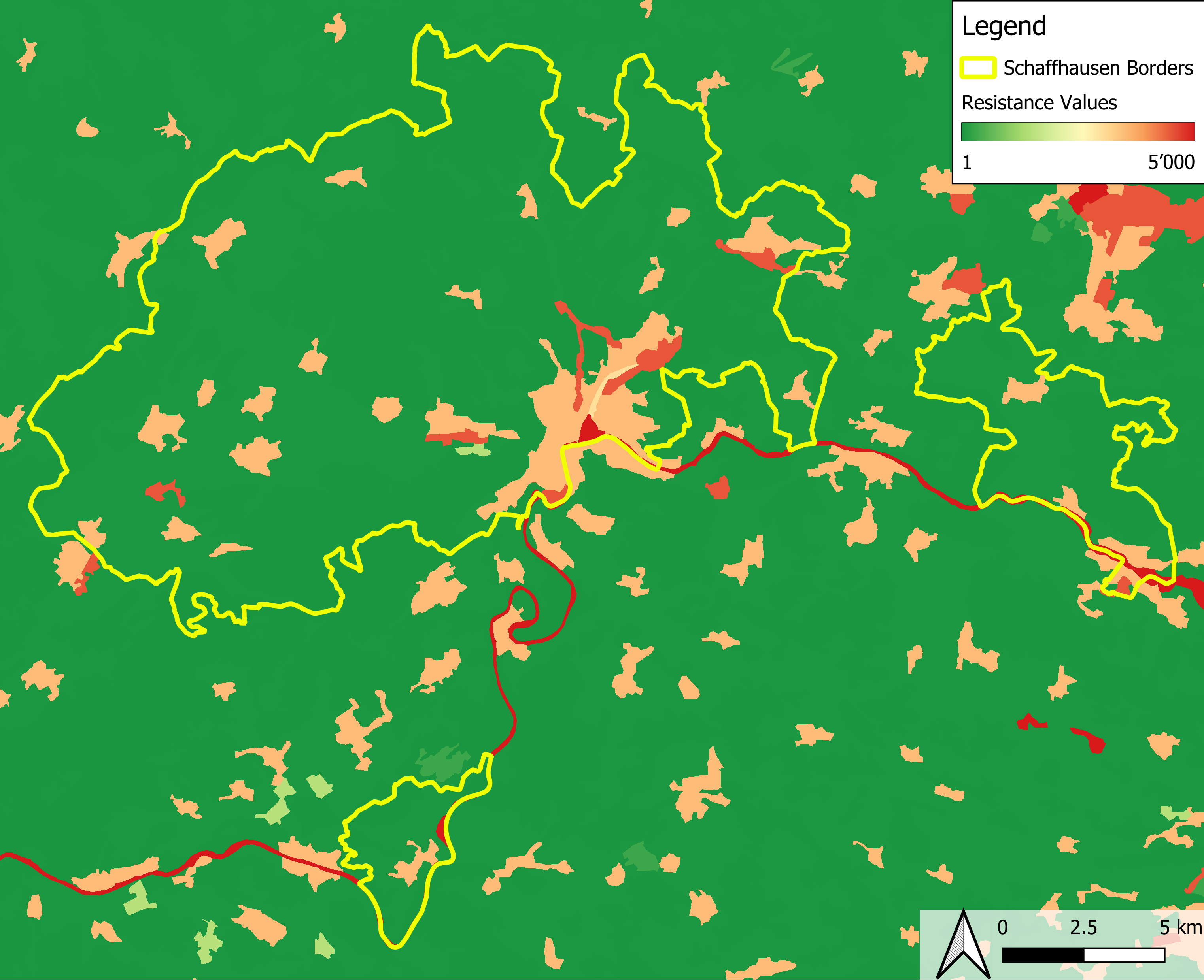
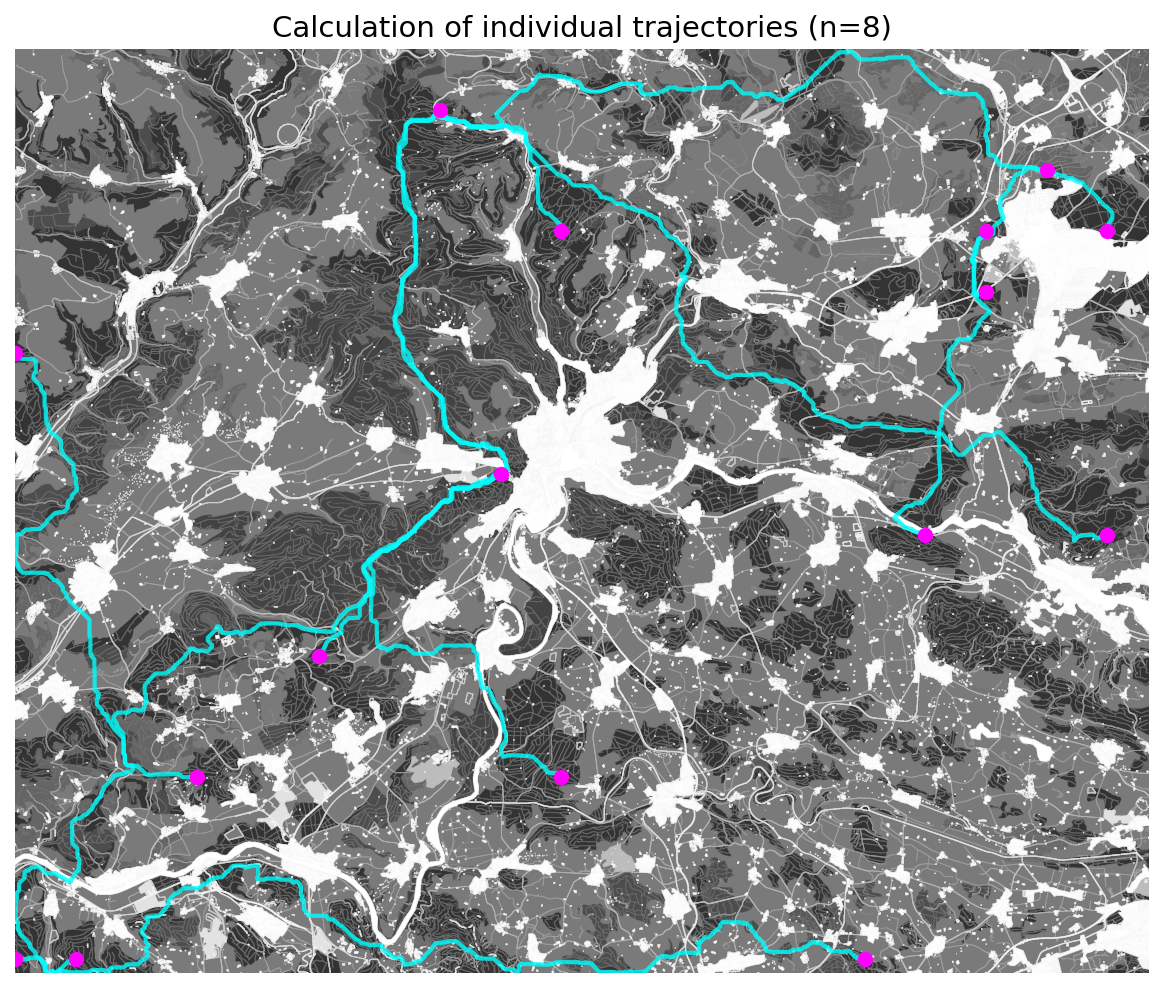
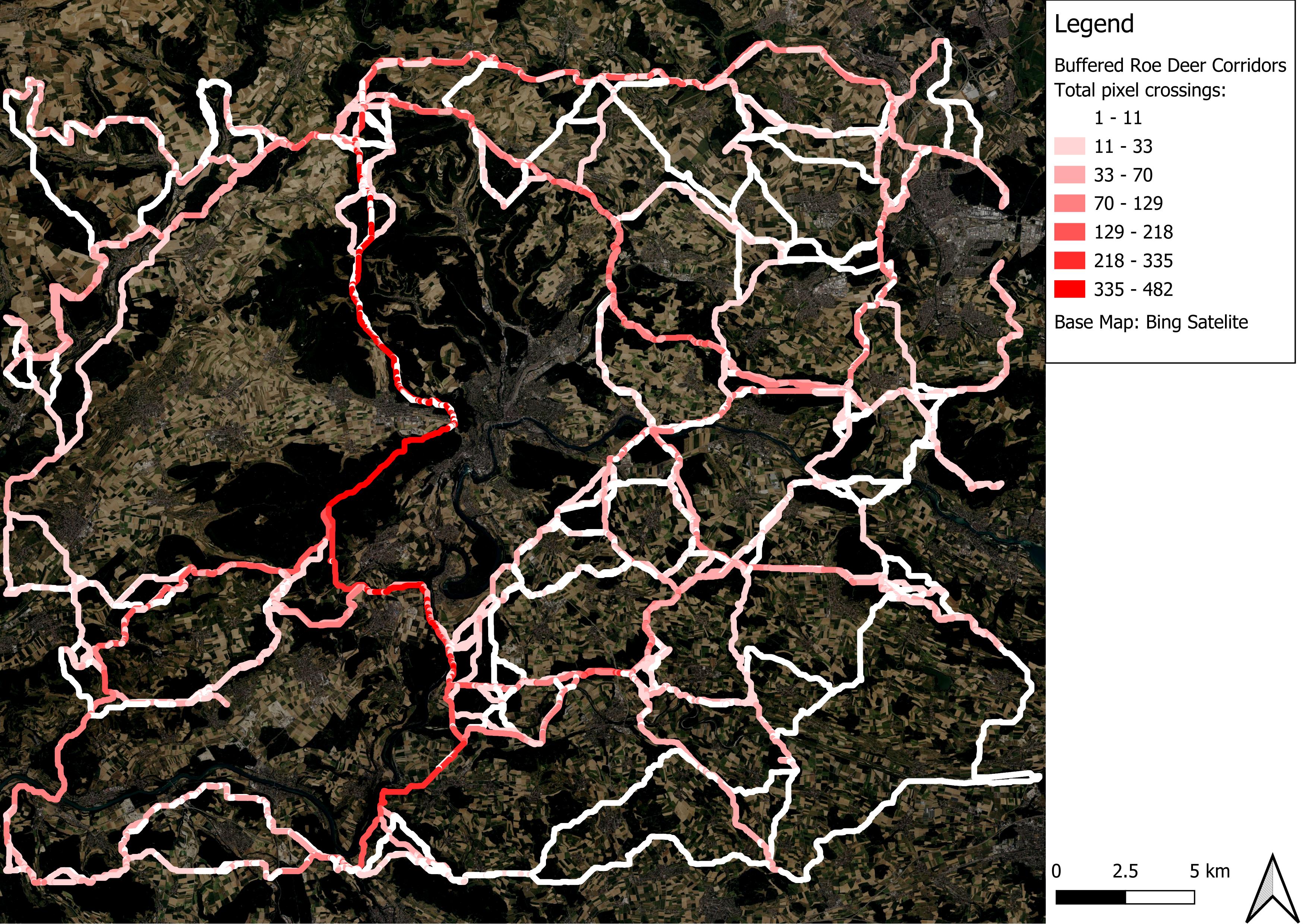
The modeled connectivity network (Figure 5) reveals that the landscape does not support diffuse, free-flowing movement. Instead, the path geometry exhibits a distinct “dendritic” or spider-web topology. This pattern indicates that movement is severely constrained by the high-resistance zones identified in the resistance surface (Figure 4).
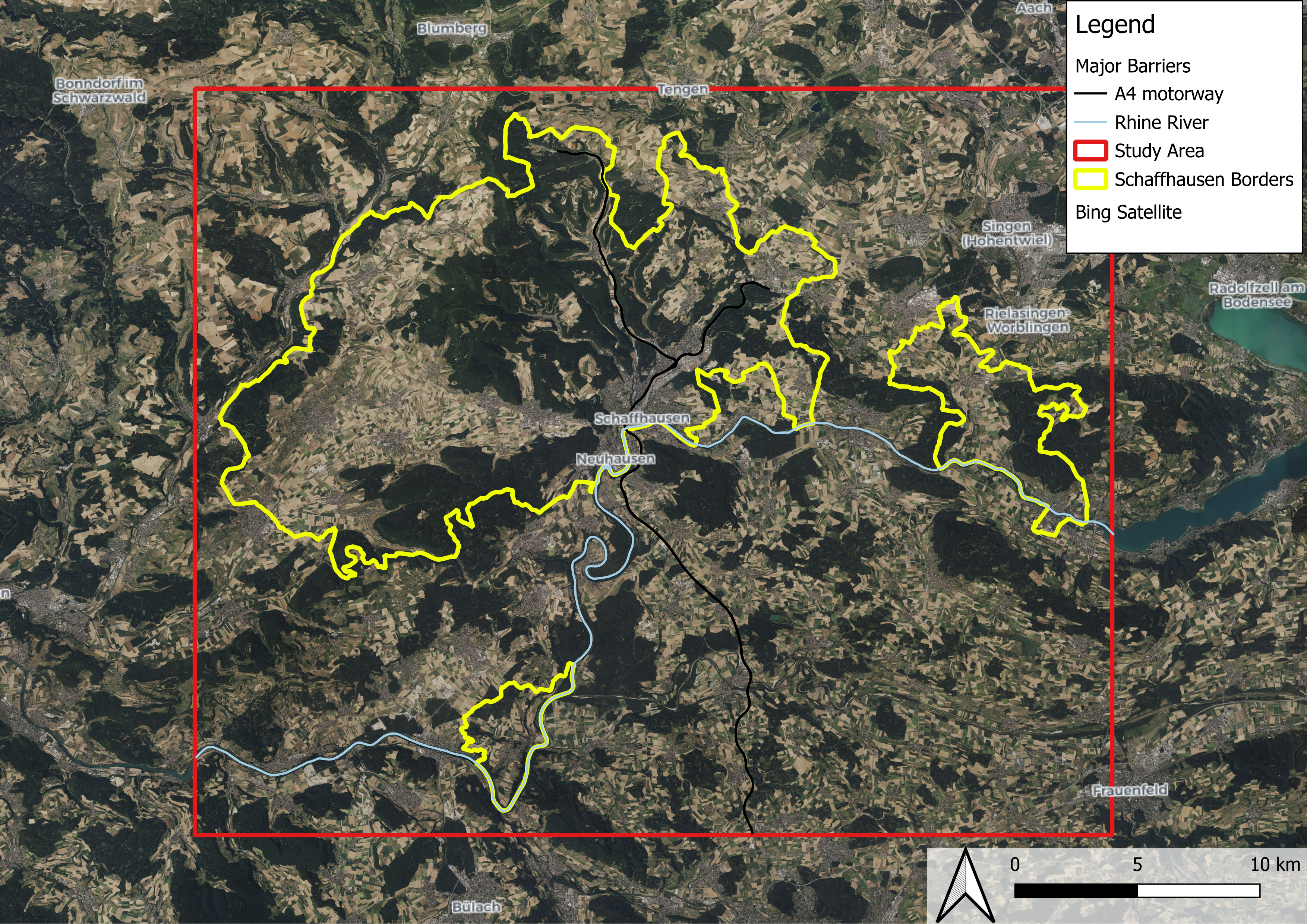
A primary finding is the identification of a significant North-South funnel located to the west of the Schaffhausen urban agglomeration. This “western corridor” appears to be the only functional biological link connecting the German habitats in the north (Baden-Württemberg) with the Swiss plateau in the south for this region. This distinct channeling effect is driven by two landscape factors:
Landscape Composition: The intense agricultural activity in the Klettgau region and the abundance of specific coniferous forest structures, which offer less optimal cover than dense mixed forests, constrain wildlife into specific routes.
Impermeable Blockades: The City of Schaffhausen combined with the adjacent A4 motorway acts as a massive barrier, effectively severing eastward movement.
Consequently, the high path density observed in these corridors (red lines in Figure 5) does not represent “preferred” habitat, but rather obligatory passage. As noted by (Haddad et al. 2015), such reliance on singular, high-intensity connections reduces the resilience of the metapopulation, the blockage of a single bottleneck (e.g., by new construction) could disproportionately isolate large habitat areas.
The Role of Infrastructure and Settlements
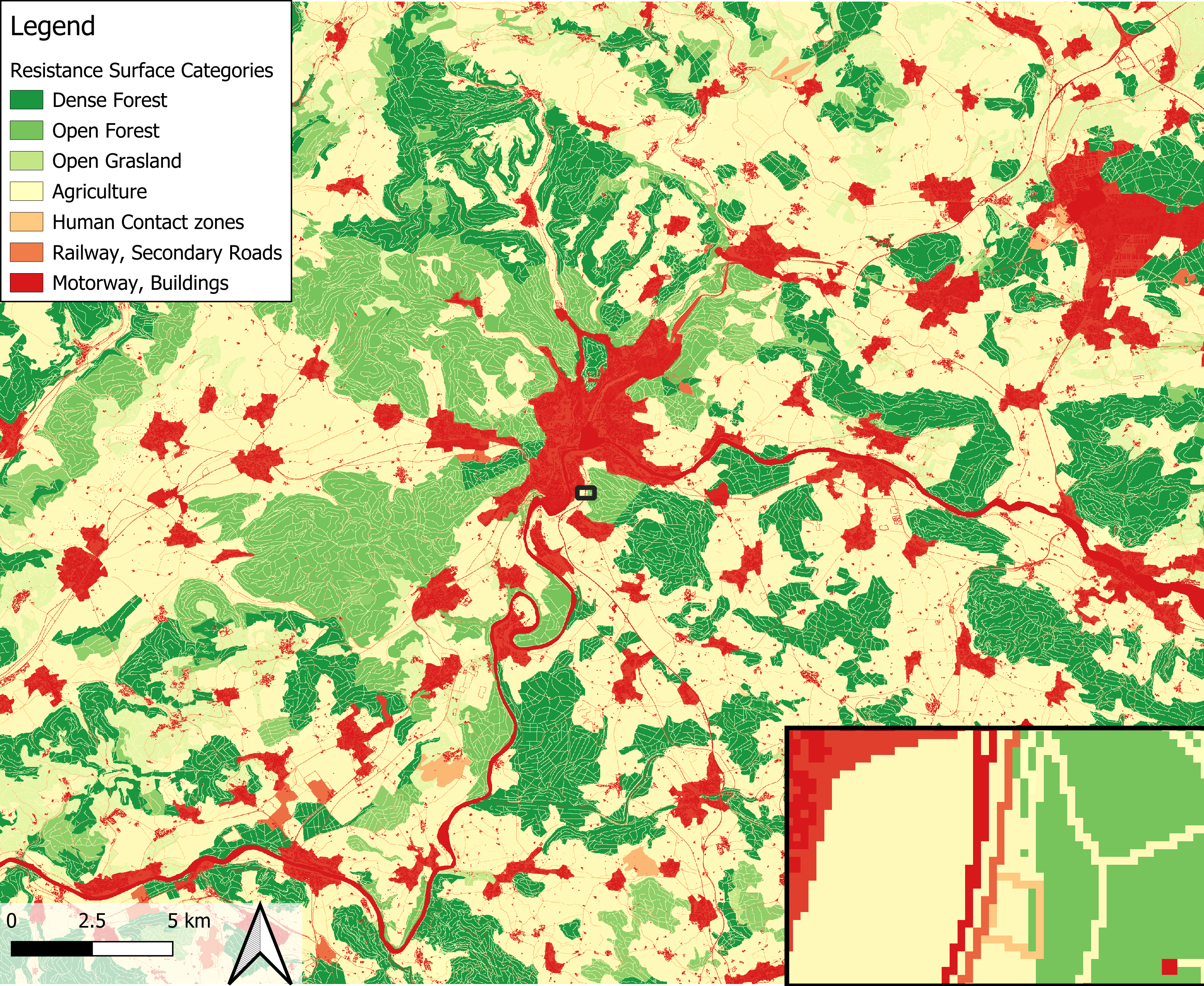
The spatial distribution of critical bottlenecks (Figure 6) confirms that linear barriers, specifically the A4 highway and the Rhine river, constitutes a primary limitation to connectivity. The model successfully captures the “Barrier Effect”, where calculated paths run parallel to highways or the Rhine river for long distances, searching for a gap with lower resistance. The clustering of bottlenecks where high movement intersects with high resistance values (\(\ge 3000\)) confirms these as conflict zones where biological needs collide with anthropogenic land use.
However, while linear barriers create specific conflict points, the model suggests that settlement boundaries are the dominant force shaping the overall network topology. The high cost weights assigned to urban areas force the Least-Cost Paths to circumnavigate towns and cities entirely. Thus, while roads act as filters that are occasionally crossed, settlements act as obstacles that dictate the macro-structure of the wildlife corridors.
Spatial Analysis of Conflict Zones
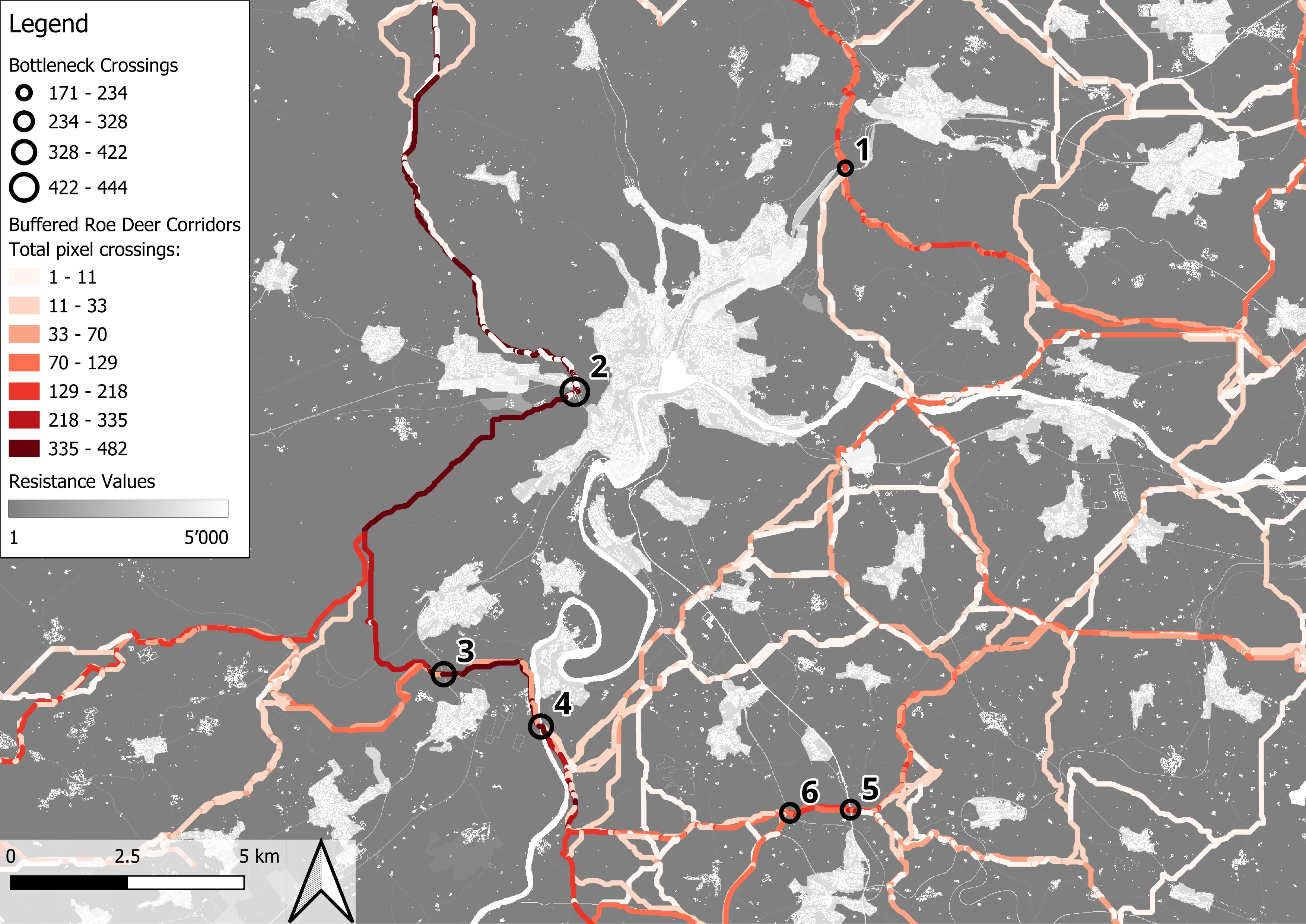
A quantitative summary of the most critical pinch points is presented in Table 1. The spatial distribution highlights specific conflict zones:
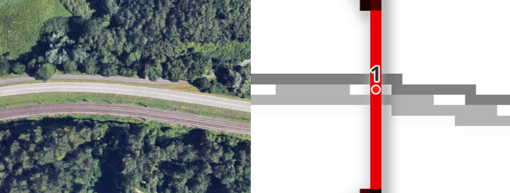
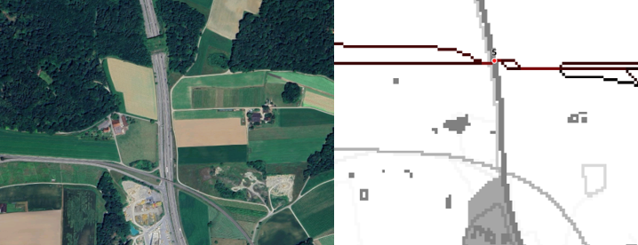
Bottleneck 1 (Thayngen) Located along the A4 motorway between Schaffhausen and Thayngen, this point represents a critical constriction where the transport infrastructure creates a continuous, high-resistance barrier. The barrier effect is compounded by the railway line running parallel to the motorway.
Despite the high anthropogenic resistance, the model identifies this location as the optimal local crossing point. This is due to the presence of two opposing forest patches that approach the infrastructure closely on both sides (see Figure 7). Ecologically, this minimizes the distance Roe Deer must travel through open, unprotected terrain. While the crossing entails significant mortality risk and energetic cost, the immediate availability of protective cover makes it the “least-cost” option compared to the surrounding open grass landscape.
At the moment, there are only deer warning signs for drivers, which suggests that collisions between cars and deer do indeed occur frequently at this location. Therefore, a wildlife underpass at this location would be highly recommended, as it would significantly improve the north-south connections of the wildlife corridors.
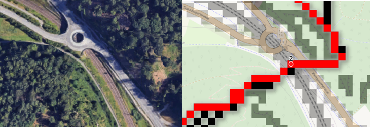
Bottleneck 2 (Western Corridor) The Beringen Constriction Bottleneck 2 recorded the highest crossing intensity of the entire network. The model identified this location as the sole functional link connecting the northern and southern populations within the western sector (Klettgau). Spatially, the corridor aligns with a narrow strip of forest sandwiched between a primary road, a railway line, and the Beringen settlement edge.
While the LCP algorithm identified this as an optimal path based on land cover (forest), a closer inspection of the topography reveals a critical potential barrier. As shown in Figure 8 (Right), the OpenStreetMap data indicates cliffs (toothed lines) running parallel to the infrastructure. The discontinuity of the cliff features in the vector data allowed the algorithm to find a “gap” beside the cliff. However, this is not very realistic, as there is usually still very steep terrain next to a cliff, which is also very difficult for Roe deer to overcome. Because the resistance surface was derived primarily from land cover (2D), the steep vertical gradients of these regions were likely underestimated. In reality, the topographic slope may render this corridor impassable for Roe Deer.
If this corridor is indeed impassable due to topography, the western sector suffers from complete functional isolation. The only alternative for wildlife would be to traverse the open, higher-resistance agricultural plains of the Klettgau, which entails significantly higher mortality risks. This highlights the importance of integrating a Digital Elevation Model (DEM) in future iterations to account for slope-based resistance.
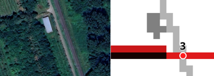
Bottleneck 3 (Jestetten-Lotstetten) This location highlights a limitation regarding the weighting of resistance parameters. The model identifies the railway line as a critical bottleneck due to the high resistance value assigned to rail infrastructure (3000). However, this likely represents an overestimation of the barrier effect. Unlike motorways, where traffic noise and collision risk are continuous, regional railway traffic is intermittent. Physically, standard tracks (absent of noise protection walls) present negligible obstruction to Roe Deer. Consequently, the model treats this railway as a “hard barrier” similar to a highway, whereas in reality, it likely possesses a much higher permeability. This finding suggests that future model iterations should refine the input sensitivity to distinguish between high-speed fenced rail lines and permeable regional tracks, potentially lowering the cost for the latter to shift focus toward high-risk roadways.
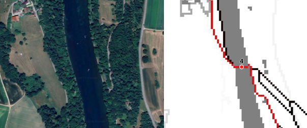
Bottleneck 4 (Rhine) The Rhine River functions as the primary linear barrier separating the northern and southern sub-populations of the canton. While Roe Deer are capable of swimming, the high flow velocity and steep, anthropogenically modified banks create high resistance values throughout the river course.
The model identifies the location in the south of Rheinau (Figure 10) as the primary connectivity link across this barrier. This selection is driven by two landscape metrics:
River Morphology: It represents one of the narrowest sections of the Rhine in the study area.
Land Cover Continuity: As seen in the aerial comparison, dense riparian forest extends to the riverbank on both sides.
This creates a “stepping stone” effect where the exposure to open terrain is minimized. From a conservation planning perspective, this location represents the most effective site for restoring functional connectivity, whether through bank renaturation to facilitate swimming or the construction of a dedicated wildlife crossing structure.
Bottleneck 5 (Schneitenberg / Andelfingen) This location serves as a critical “Ground Truth” validation for the entire connectivity model. Located along the A4 motorway near Andelfingen, the model identified a high-priority crossing point where the motorway bisects two expansive forest blocks.
The LCP algorithm selected this specific coordinate because it minimizes the crossing distance over the high-resistance road surface while maximizing the proximity to protective cover on both sides. As illustrated in the split-view comparison (Figure 11), this modeled trajectory aligns precisely with the existing Schneitenberg Wildlife Overpass.
Because the specific low resistance of the bridge was not explicitly hard-coded into the resistance surface (i.e., the model viewed it as a standard road segment), this result confirms the model’s high predictive power. It demonstrates that the geometric approach successfully identifies the same optimal ecological links that have been prioritized by real-world landscape planning. The model correctly “predicted” the location of a conservation structure based solely on landscape connectivity principles.
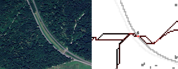
Bottleneck 6 (Marthalen / Andelfingen) Similar to Bottleneck 3, the identification of this crossing is partially driven by the high resistance value assigned to railway infrastructure (\(R=3000\)). However, unlike the isolated rural track at Jestetten, this location represents a larger barrier system. As visible in the aerial imagery (Figure 12), the railway runs in immediate proximity to a secondary cantonal road. While the railway itself may be permeable, the combined width of the multi-modal transport corridor significantly increases the “exposure time” for crossing wildlife, validating its classification as a risk zone.
Despite the confirmed risk, this location represents a lower priority for structural intervention compared to the massif barriers at the A4, Rhine river or “western Corridor” (Klettgau). In those locations, functional connectivity is completely severed. At Bottleneck 6, permeability likely still exists during periods of low traffic. Therefore, mitigation resources should be allocated to the A4, Rhine and western Corridor crossings first.
Model Plausibility and Real-World Relevance
Cross-Verification
The plausability of the modell is supported by a spatial cross-verification with an independent traffic accident risk model provided by the ZHAW Institut für Umwelt und Natürliche Ressourcen (IUNR) (“Prävention von Wildtierunfällen Auf Verkehrsinfrastrukturen” n.d.).
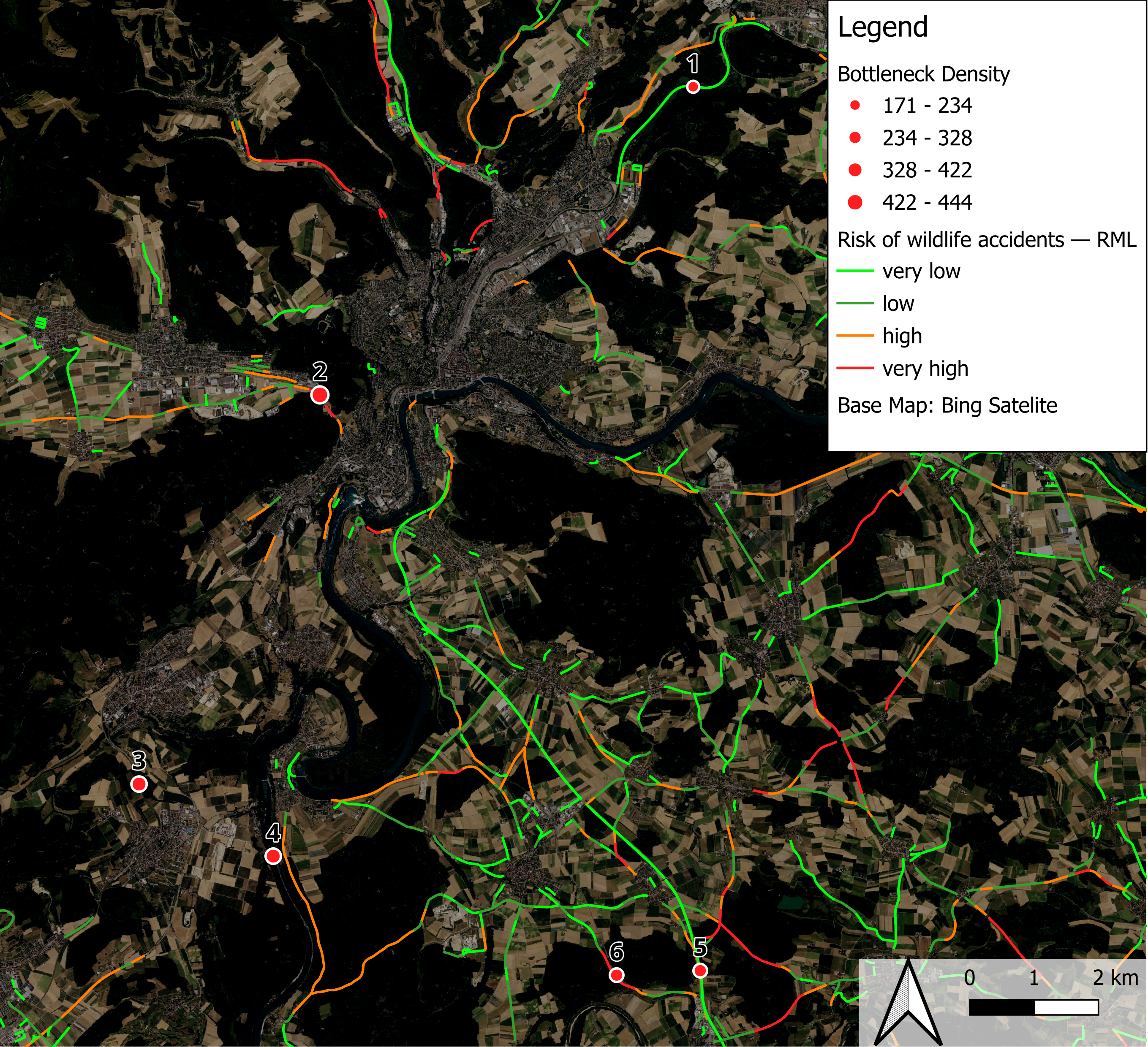
Figure 13 visualizes the spatial distribution of the modeled high-risk bottlenecks (Red Dots) against the regional infrastructure network. A visual inspection reveals a nuanced relationship between the connectivity model (LCP) and the accident risk model (RML).
High-Risk Alignment: A strong correlation is observed at Bottleneck 2 and Bottleneck 6. Bottleneck 2 coincides with a “very high” risk segment (red line), confirming the model’s prediction of high animal movement pressure, although local topological constraints may severely limit the feasibility of a wildlife overpass at this specific location. Similarly, while Bottleneck 6 is centered on a railway line, the immediately adjacent road segment is classified as “very high” risk, suggesting a corridor that spans both infrastructure types.
Mitigated or Latent Risk: In some instances, the connectivity model identifies bottlenecks where the recorded accident risk is “very low” (light green lines). Bottleneck 5, located on the A4 motorway, is classified as low risk, this is likely attributable to an existing wildlife overpass at this location which successfully mitigates collisions while confirming the high connectivity value of the segment. Bottleneck 1 is also situated on a low-risk road segment, though the presence of roe deer warning signs suggests a known hazard potential that may not be fully reflected in the accident statistics.
Non-Road Barriers: Finally, the model identifies barriers outside the road network. Bottleneck 3 is located on a railway line, and Bottleneck 4 is situated on the Rhine river. As the RML dataset is specific to road traffic accidents, these significant landscape barriers do not possess a corresponding risk classification in the reference model.
Ground Truthing
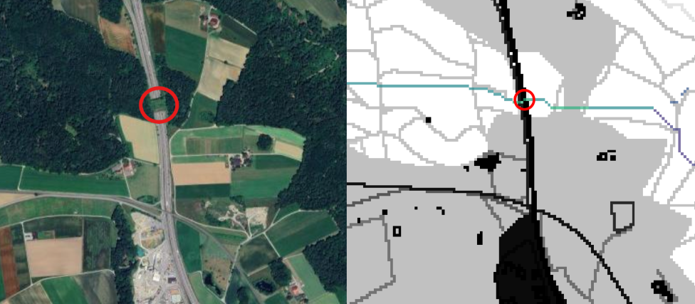
A critical “ground truth” validation is provided by the specific analysis of Bottleneck 5 (identified in Table 1). The Least-Cost Path (LCP) model pinpointed this location as a high-priority crossing point based on the underlying resistance surface without explicit prior programming of the specific infrastructure.
Figure 14 presents a direct comparison between the physical reality and the simulation output. The left panel displays satellite imagery of the Schneitenberg wildlife overpass spanning the A4 motorway. The right panel illustrates the corresponding LCP analysis. As highlighted by the red circle, the modeled path does not traverse the highway barrier arbitrarily. Instead, the pathfinding algorithm funnels the route effectively to the precise coordinates of the existing bridge.
The fact that the algorithm independently navigated the path to the location where civil engineers previously sited a green bridge serves as a strong indicator of model robustness. It suggests that the resistance surface correctly captures the landscape features that naturally guide Roe Deer to the most energetically efficient crossing points.
Methodological Reflection and Limitations
Computational Artifacts: Path Dispersion
A technical challenge encountered during the LCP analysis was the “path smearing” effect. Because the algorithm calculates optimal routes on a pixel-by-pixel basis, distinct paths often crossed linear barriers in close proximity but on different pixels. This resulted in a spatial dispersion of the crossed pixels, leading to an initial underestimation of traffic intensity at specific bottlenecks. Future iterations of the model could mitigate this by applying a focal statistics filter (e.g., a Kernel Density Estimator) to the traffic raster. This would aggregate adjacent pixel values into a coherent “corridor width”, better representing the biological reality of animal movement zones rather than exact linear trajectories.
Temporal Stationarity
A fundamental limitation of the model is its static nature. The landscape is represented as a fixed snapshot based on the CLC 2018 and current OSM datasets. Consequently, the model does not account for temporal dynamics, such as:
Seasonal Variations: The permeability of agricultural land changes drastically between harvest (high visibility/risk) and peak growth (high cover).
Diurnal Traffic Patterns: The resistance of roads is treated as constant, whereas in reality, traffic volume fluctuates significantly between day and night, influencing crossing success probabilities.
In addition, future improvements could better adapt the preferred areas of deer. Since deer tend to stay at the edge of the forest, the model could be made even more accurate by explicitly selecting these forest edges as starting points for the LCP calculation.
Data Granularity and Topography
The model’s precision is intrinsically linked to the resolution of the input data.
Topographic Simplification: The exclusion of slope data represents a geometric simplification. While this approach is valid for the relatively flat agricultural plateau of the Klettgau, it likely overestimates connectivity in the rugged Randen massif, where steep gradients impose significant energetic costs on roe deer. As described in the report, the lack of Slope data has created a bottleneck that appears impossible for deer to cross due to the cliffs.
Data Heterogeneity: While OpenStreetMap provides high-resolution data for infrastructure, the attribute completeness (e.g., fence heights or exact forest types) varies. Proprietary data (e.g., LiDAR-derived vegetation height models) would be required to model micro-habitat features, such as understory density, which significantly influences shelter availability.
Sensitivity Analysis
Finally, no systematic sensitivity analysis was conducted. The resistance values were assigned based on expert literature, but it remains unquantified how sensitive the location of the predicted corridors is to minor changes in these weights (e.g., varying road cost between 1000 and 5000). As shown in the project some cost values should be improved and set to a more realistic value.